These days, papers such as du Plessis et al. (NIPS2014)¹ and Sakai et al. (ICML2017)² refers optimality of convergence rates of their learning methods. The convergence rate $O(n^{-\frac{1}{2}})$ is referred to as optimal (parametric) convergence rate for classification. In this article, I investigate why this is optimal for empirical risk minimization.

Most of the parts in this article try to describe intuition of Mendelson’s technical report³. I tried to explain as intuitive as possible, but sometimes sacrificed rigidness of discussion. It would be better to utilize this article as an auxiliary material to read Mendelson’s report.

Prologue

$$ \newcommand{\argmax}{\mathrm{argmax}} \newcommand{\argmin}{\mathrm{argmin}} \renewcommand{\hat}{\widehat} $$

In statistical machine learning, there are mainly the following two types of problems:

1. estimation of a true target (function learning)
2. selection of a criterion minimizer (agnostic learning)

Examples for the first problem is density estimation and squared mutual information⁴. These problems have (unknown) true targets, and their goal is to estimate true targets by statistical methods. In statistical estimation, first we have a model $\mathcal{F}$ and loss $L$ written by the expectation. The expectation is usually replaced with samples and we obtain empirical version $\hat{L}$. Let

• $f^* = \argmin_{f \in \mathcal{F}} L(f)$
• $\hat{f} = \argmin_{f \in \mathcal{F}} \hat{L}(f)$

then we estimate $f^*$ by $\hat{f}$. However, our model class $\mathcal{F}$ does not always include the true target $f^\dagger$ (when model is mis-specified). Thus we need to consider

• estimation error: error between $\hat{f}$ and $f^*$, originating from sample approximation and optimization
• approximation error: error between $f^*$ and $f^\dagger$, originating from model specification

On the other hand, usually we only need to consider estimation error in the second problem. A common example is classification. Basically there does not exist a unique target, rather our goal is to select the best model. In classification, our goal is to obtain the model with minimum errors, which is not necessarily a classifier with zero errors⁵. The goal is often achieved by the empirical risk minimization.

In both cases, it still remains the same what we need to do to obtain a model, i.e., minimizing estimation error, but there is a subtle difference in philosophy. Now let’s move on to discussion of convergence rates (of the estimation error).

Notations

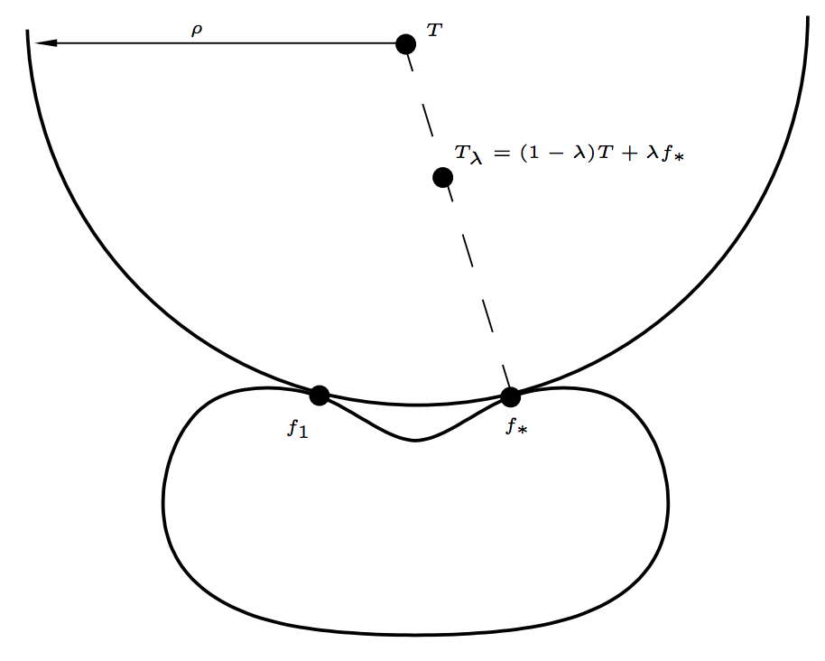
Afterwards, I mainly refer to the technical report written by Mendelson³ to discuss optimality of convergence rates. We consider function learning problem, where the learner is given a random sample $\{X_i\}_{i=1}^k \sim \mu$ and $\{T(X_i)\}_{i=1}^k$ ($T$: target function). Assume that $E$ is a reasonable normed space of random variables on $(\Omega,\mu)$, a loss function is connected to the norm of $E$ (e.g., $p$-loss⁶ for $L_p$ space), $F \subset E$ is a “small” model class where $T$ has more than one best approximation. Let $N(F,E)$ be the set of functions in $E$ that have more than one best approximation in $F$. Let $f_* \in F$ be a fixed best approximation of $T$ (chosen one arbitrarily), and $T_\lambda = (1 - \lambda)T + \lambda f_*$.

(the figure is borrowed from Mendelson’s report)

Later, for $\lambda_k \sim 1/\sqrt{k}$, $T_{\lambda_k}$ appears to be a “bad” target function, i.e., $$ \mathbb{E}_X \mathbb{E}\left( \ell(\hat{f},T_{\lambda_k}) \mid X_1,\dots,X_k \right) - \inf_{f \in F} \mathbb{E} \ell(f,T_{\lambda_k}) \ge \frac{c}{\sqrt{k}}, $$ where $\hat{f}$ is the empirical risk minimizer and $c$ is a constant depending only on $F$, $\ell$ and $E$.

Let $P_kg = \frac{1}{k} \sum_{i=1}^k g(X_i)$, $Pg = \mathbb{E}_Xg$⁷. Let $\mathcal{L}(f) = \ell(f,T) - \ell(f_*,T)$ and $\mathcal{L}_\lambda(f) = \ell(f,T_\lambda) - \ell(f_*,T_\lambda)$ be the excess loss functional w.r.t. $T$ and $T_\lambda$, respectively.

Main Theorem

The following theorem is main statement of Mendelson’s technical report, which tells us what is the optimal convergence rate, or the lower bound for the empirical risk minimization.

Theorem 1.2 Let $2 \le p \le \infty$ and $E = L_p(\mu)$. Assume that $F \subset E$ is a $\mu$-Donsker class of functions bounded by $1$, let $R > 0$ and assume that $\mathcal{T} \subset E \cap B(0, R)$ is convex and contains $F$. If $\ell$ is the $p$-loss function and $\mathcal{T} \cap N(F,E) \ne \emptyset$, then for $k \ge k_0$, $$ \sup_{T \in \mathcal{T}}\left( \mathbb{E}_X \mathbb{E}\left( \ell(\hat{f}, T) \mid X_1, \dots, X_k \right) - \inf_{f \in F} \mathbb{E}\ell(f,T) \right) \ge \frac{c}{\sqrt{k}} , $$ where $c$ and $k_0$ depend only on $p$, $F$ and $R$.

This theorem states that the empirical risk minimizer $\hat{f}$ cannot do better than $O(1/\sqrt{k})$ against a certain target function. In other words, even if the empirical risk minimizer is obtained, its excess risk is more than $O(1/\sqrt{k})$ for a certain target function. Thus $O(1/\sqrt{k})$ is said to be optimal convergence rate for ERM. If we want to obtain faster rate, we need to make stronger assumptions jointly on density, loss function and model class, which is hardly satisfied in practice.

Outline of Proof

The following figure hopefully clarifies relationships between theorems/lemmas in Mendelson (2008).

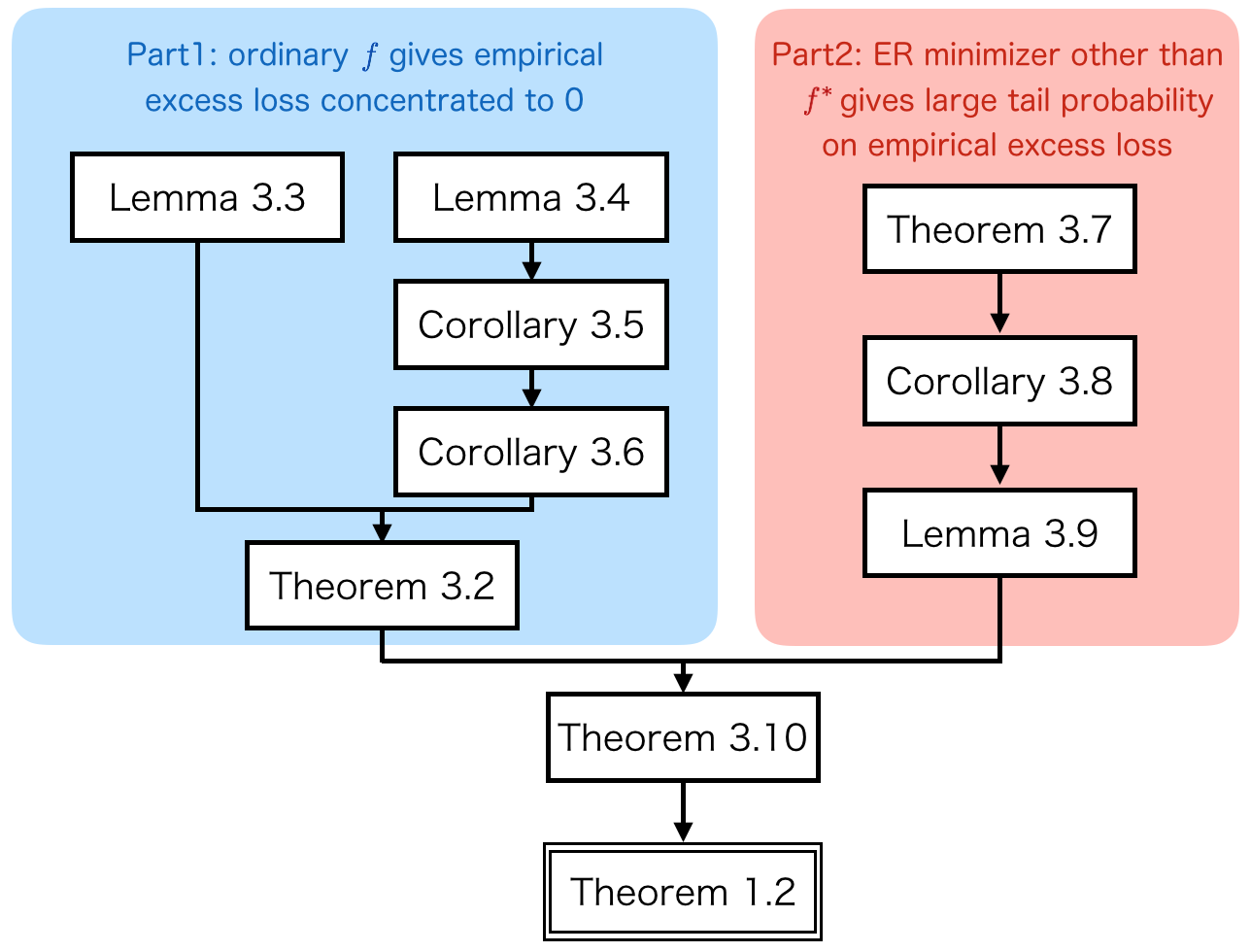
In Part1, it is shown that $f$ with small expected excess loss $P\mathcal{L}_{\alpha/\sqrt{k}}(f) \le \beta/\sqrt{k}$ gives small empirical excess loss: $|P_k\mathcal{L}_\lambda(f)| \le C/\sqrt{k}$ with high probability, say $\frac{5}{6}$ (Theorem 3.2). In Part2, “bad” target $T_\lambda$ is constructed when $\lambda \sim \alpha/\sqrt{k}$: $P_k\mathcal{L}_\lambda(f) \le -C/\sqrt{k}$ with some probability, say $\frac{1}{4}$ (Lemma 3.9), which is larger than $1 - \frac{5}{6} = \frac{1}{6}$ (the probability of $|P_k\mathcal{L}_\lambda(f)| > C/\sqrt{k}$ even if $P\mathcal{L}_\lambda(f) \le r$). Hence, with probability at least $\frac{1}{12}$ over choice of samples $\{X_i\}_{i=1}^k$, “bad” target $T_\lambda$ gives $$ P\mathcal{L}_\lambda(f) > r \sim \frac{\beta}{\sqrt{k}}, $$ which gives a simple proof of Theorem 1.2⁸. I summarize the above intuition in the following animation.

The key ingredient is Berry-Esséen Theorem (Theorem 3.7), which gives convergence rate of the central limit theory. Afterwards, I will go through some important parts in the proofs individually, focusing on parts difficult to follow (for me).

Theorem 3.2 (main body of Part1)

The main claim of Part1 is stated in the following theorem.

Theorem 3.2 Let $F$ be a classof functions that is compatible with the norm of $E$ and set $F_{\lambda,r} = \{f \mid P\mathcal{L}_\lambda(f) \le r\}$. For every $\alpha,u > 0$ there is an integer $k_0$ and $\beta \in (0,u]$ such that for $k \ge k_0$, with probability $\frac{5}{6}$, $$ \sup_{f \in F_{\alpha/\sqrt{k},\beta/\sqrt{k}}} |P_k\mathcal{L}_{\alpha/\sqrt{k}}(f)| \le \frac{2u}{\sqrt{k}}. $$

Intuitively, for $\lambda \sim \alpha/\sqrt{k}$, if the expected excess loss $P\mathcal{L}_\lambda(f) \le \beta/\sqrt{k}$, then the empirical excess loss $|P_k\mathcal{L}_\lambda(f)| \le 2u/\sqrt{k}$ with high probability. This fact combined with Part2 (Lemma 3.9) shows for a certain case $P_k\mathcal{L}_\lambda(f) \le -C/\sqrt{k}$, and that $P\mathcal{L}_\lambda(f) > \beta/\sqrt{k}$.

Let’s follow the proof using Lemma 3.3. Actually, most of the parts of the proof of Theorem 3.2 in the technical report is clear except Equation (3.2), which I want to clarify here: $$ \begin{align} \sup_{f \in F_{\lambda,r}} |P_k\mathcal{L}_\lambda(f)| & \le \sup_{f \in F_{\lambda,r}} |P\mathcal{L}_\lambda(f)| + |(P_k - P)\mathcal{L}_\lambda(f)| \\\\ & \le r + \sup_{f \in F_{\lambda,r}} |(P_k - P)\mathcal{L}_\lambda(f)| \\\\ & \le r + \mathbb{E}_X \sup_{f \in F_{\lambda,r}} |(P_k - P)\mathcal{L}_\lambda(f)| + \frac{c_\text{conc}}{\sqrt{k}}, \end{align} $$ where the first inequality is the triangular inequality, the second inequality is given by the condition $f \in F_{\lambda,r}$ and the third inequality is given by concentration inequalities, such as McDiarmid’s inequality: $$ P_k\Psi \le P\Psi + \sqrt{\frac{M\log(2/\delta)}{2k}} \qquad \text{with probability at least $1-\delta$}, $$ where for any $\delta \in (0, 1)$, $M$ is a constant depending on boundedness of a functional $\Psi$. Here we set $\Psi = \sup|(P_k - P)\mathcal{L}_\lambda(f)|$ and $\delta = \frac{1}{6}$, then $c_\text{conc}$ is obtained as $\sqrt{M\log(12) / 2}$.

The following part of the proof of Theorem 3.2 is not so difficult. In fact, the confidence term $c_\text{conc}/\sqrt{k}$ is missing on the right hand side of Equation (3.2), I think. Fortunately, the order of the confidence term is still $1/\sqrt{k}$, we can obtain the same upper bound with the original Theorem 3.2.

Berry-Esséen Theorem (Theorem 3.7) → Corollary 3.8

Berry-Esséen Theorem gives actual convergence rate of the central limit theory.

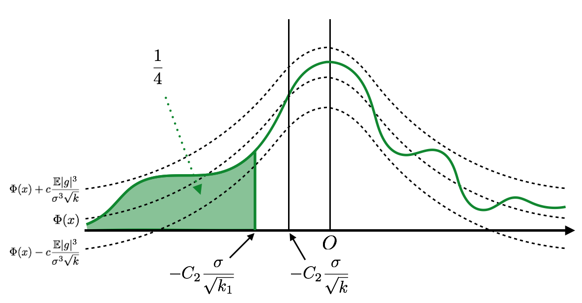
Theorem 3.7 (Berry-Esséen Theorem) Let $\{\xi_i\}_{i=1}^k$ be i.i.d. random variables with mean 0 and variance $\sigma^2$, $F_k(x)$ be the distribution function of $\frac{1}{\sigma\sqrt{k}}\sum_{i=1}^k\xi_i$ and $\Phi(x)$ be the distribution function of the standard Gaussian. Then, for some constanct $c$, $$ \sup_{x\in\mathbb{R}}|F_k(x) - \Phi(x)| \le c\frac{\mathbb{E}|\xi_1|^3}{\sigma^3\sqrt{k}}. $$

B-E Theorem states $F_k(x)$ converges to $\Phi(x)$ in distribution, and its rate is $c\mathbb{E}|\xi_1|^3/\sigma^3\sqrt{k}$. Using this theorem, we can tell the left tail probability of $F_k(x)$.

Corollary 3.8 Let $g$ be a random function with variance $\sigma^2$ and finite third moment. Then, there exists $k_1$ depending only on $\sigma$ and $\mathbb{E}|g|^3$, and a constant $C_2$ such that for all $k \ge k_1$, with probability at least $\frac{1}{4}$ over the choice of $\{X_i\}_{i=1}^k$, $$ \frac{1}{k}\sum_{i=1}^kg(X_i) \le \mathbb{E}g - C_2\frac{\sigma}{\sqrt{k}}. $$

This corollary can simply be obtained by setting $C_2$ as the following figure.

The green line shows the distribution function of $\frac{1}{\sigma\sqrt{k}}\sum_{i=1}^k(g(X_i)-\mathbb{E}g)$. Thus, its left tail probability for $k \ge k_1$ is slightly larger than $\frac{1}{4}$. The choice of value $\frac{1}{4}$ does not have special meaning, just saying $g$ goes to “very negative” with certain probability.

Construction of “Bad” Target (main body of Part2)

Back to Theorem 3.2, most of functions $f$ with small expected excess loss $P\mathcal{L}_\lambda(f) \le r$ gives empirical excess loss concentrated on $0$, that is, $|P_k\mathcal{L}_\lambda(f)| \le 2u/\sqrt{k}$ with high probability. In this section, a “bad” target, i.e., $P_k\mathcal{L}_\lambda(f) \le -C/\sqrt{k}$ even if $P\mathcal{L}_\lambda(f)$ is small. Such a bad target results in the lower bound of ERM convergence rate $O(1/\sqrt{k})$. To construct a bad target, Corollary 3.8 will be applied for $g = \mathcal{L}_\lambda(f)$. Since $\mathbb{E}\mathcal{L}_\lambda(f) \sim 1/\sqrt{k}$ can be confirmed, $P_k\mathcal{L}_\lambda(f) \le -C/\sqrt{k}$ will be obtained.

Recall that we can take $T \in N(F,E)$ (see the supremum condition in Theorem 1.2), which means $T$ has more than one best approximator. Let’s take $f_1$ as other (fixed) approximator than $f_*$ (please refer to the figure in Notation).

Lemma 3.9 There exist constants $C_3$, $C_4$, $\lambda_0$ and $k_1$ depending only on $\rho=\|T-f_*\|$, $\|\phi\|_\text{lip}$, $\|\ell\|_\text{lip}$, $D_3=\sup_{f \in F}\|T-f\|_{L_3(\mu)}$, $\Delta=\mathbb{E}|\mathcal{L}(f_1)|$ such that for all $\lambda \in [0, \lambda_0]$,

1. $\mathbb{E}\mathcal{L}_\lambda(f_1) \le 2\lambda\rho\|\phi\|_\text{lip}$
2. $\text{var}(\mathcal{L}_\lambda(f_1)) \ge \Delta^2 / 4$
3. $\forall k \ge k_1, \lambda_k \ge \min\{\lambda_0, C_3/\sqrt{k}\}$, with probability at least $\frac{1}{4}$, $P_k\mathcal{L}_\lambda(f_1) \le -\frac{C_4}{\sqrt{k}}$

The first statement holds only for best approximators of $T$: $$ \begin{align} \mathbb{E}\mathcal{L}_\lambda(f_1) &\le \phi(\|T_\lambda - f_1\|) - \phi(\|T_\lambda - f_*\|) \\\\ &= (\phi(\|T_\lambda - f_1\|) - \phi(\|T - f_1\|)) + (\phi(\|T - f_*\|) - \phi(\|T_\lambda - f_*\|)) \\\\ &\le 2\|\phi\|_\text{lip} \|T - T_\lambda\| \\\\ &= 2\lambda\|\phi\|_\text{lip}\|T - f_*\| \\\\ &= 2\lambda\rho\|\phi\|_\text{lip}, \end{align} $$ where the equality in the second line holds only for best approximators $f_1$ ($\|T - f_1\| = \|T - f_*\|$). The first inequality follows Assumption 2.1 (please refer to the original report).

The third statement follows Corollary 3.8, because $\mathbb{E}\mathcal{L}_\lambda(f_1)$ is upper bounded by $2C_3\rho\|\phi\|_\text{lip}/\sqrt{k}$ when $\lambda$ is small enough.

The points are summarized as follows.

• There is a target $T$ which has more than one best approximation.
• For such $T$, there is a target $T_{C_3/\sqrt{k}}$ which gives “very negative” empirical excess loss on the empirical minimizer.

Here, “very negative” means smaller than $-C_4/\sqrt{k}$.

Epilogue

Theorem 3.10 can simply be obtained by the combination of Theorem 3.2 and Lemma 3.9. $P_k\mathcal{L}_\lambda(f_1)$ goes to very negative with probability at least $\frac{1}{4}$ (Lemma 3.9), while it goes to very negative in the usual case (i.e., the case $P\mathcal{L}_\lambda(f) \le c_2/\sqrt{k}$) with probability at most $\frac{1}{6}$ (Theorem 3.2). Combining them, the unusual case $P\mathcal{L}_\lambda(f_1) \ge c_2/\sqrt{k}$ happens with probability at least $\frac{1}{12}$. This probability does not vanish because of Berry-Esséen Theorem. The animation in Outline of Proof hopefully describes intuition well.

Finally, taking the expectation over $\{X_i\}_{i=1}^k$ and taking the supremum of $T \in \mathcal{T}$, Theorem 3.10 reduces to Theorem 1.2.