I would like to summarize the contents of van de Geer (2000)¹ one chapter by one, which is devoted for the theory of the empirical process and the convergence rates.

In Chapter 2, the definitions of the empirical process and entropy are given.

Empirical Measure

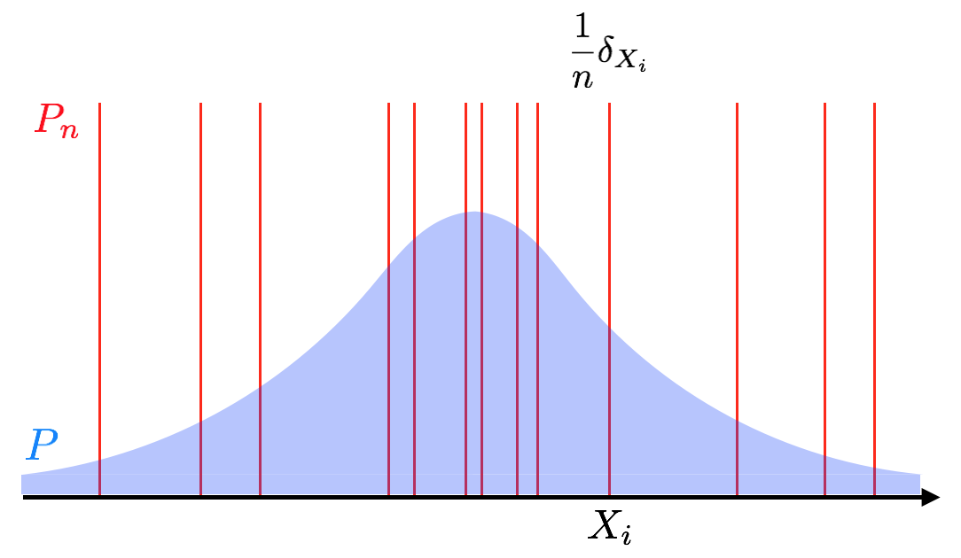
As the number of samples gets larger, the estimation error will converge to zero in many cases. This convergence property is stated by the empirical process. First, let’s begin with the definition of the empirical measure.

Let $X_1, X_2, \dots$ be independent copies of a r.v. $X$ in a probability space $(\mathcal{X}, \mathcal{A}, P)$, and $\mathcal{G} \triangleq \{g: \mathcal{X} \rightarrow \mathbb{R}\}$ be a class of measurable functions on $\mathcal{X}$. The sample average can often be seen as an empirical expectation. Let $P_n$ be the empirical measure based on $X_1, \dots, X_n$, i.e., for each set $A \in \mathcal{A}$, $$ P_n(A) \triangleq \frac{1}{n} \#\{X_i \mid X_i \in A\} = \frac{1}{n}\sum_{i=1}^n 1_A(X_i). $$ Thus, $P_n$ put mass $\frac{1}{n}$ at each $X_i$:

$$ P_n = \frac{1}{n}\sum_{i=1}^n \delta_{X_i}, $$ where $\delta_{X_i}$ is a point mass at $X_i$. The below figure describes the intuition.

Empirical Process

Now we use the notation $$ \int g dP_n \triangleq \frac{1}{n}\sum_{i=1}^ng(X_i). $$

Then, the difference between the empirical average and expectation is $$ \frac{1}{n}\sum_{i=1}^ng(X_i) - \mathbb{E}g(X) = \int gd(P_n - P). $$ The set of this quantity indexed by the class $\mathcal{G}$ is called the empirical process: $$ \left\{ \sqrt{n} \int gd(P_n - P) \right\}_{g \in \mathcal{G}}. $$

In the empirical process theory, we study the uniform convergence, i.e., the empirical process converges to zero for any $g \in \mathcal{G}$. Then we obtain the uniform law of large numbers (ULLN) and uniform central limit theorem, compared with the classical ones. They are discussed in later chapters.

Entropy

In order to investigate whether a given class satisfies the ULLN and how fast the convergence is, the complexity of the function class is needed. In the theory of nonparametric estimation, the complexity measure called entropy is often used. Afterwards, we introduce three types of entropy:

• uniform entropy
• bracketing entropy
• entropy for the supremum norm

Uniform Entropy

Let $Q$ be a measure on $(\mathcal{X}, \mathcal{A})$, and $L_p(Q) \triangleq \{g: \mathcal{X} \rightarrow \mathbb{R} \mid \int |g|^pdQ < \infty \}$ for $1 \le p < \infty$. For $g \in L_p(Q)$, write $$ \|g\|_{p,Q}^p \triangleq \int |g|^pdQ. $$ $\|\cdot\|_{p,Q}$ is referred to as $L_p(Q)$-norm. $L_p(Q)$-metric between $g_1, g_2 \in L_p(Q)$ is defined as $\|g_1 - g_2\|_{p,Q}$.

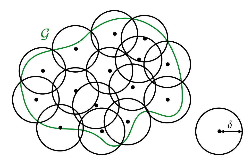
Definition 2.1 (uniform entropy) For any $\delta < 0$, consider a collection of $g_1, \dots, g_N$ such that for any $g \in \mathcal{G}$, there exists $j = j(g) \in \{1, \dots, N\}$, such that $$ \|g - g_j\|_{p,Q} \le \delta. $$ Let $N_p(\delta,\mathcal{G},Q)$ be the smallest value of $N$, which is called $\delta$-covering number Then, $$ H_p(\delta,\mathcal{G},Q) \triangleq \log N_p(\delta,\mathcal{G},Q) $$ is $\delta$-(uniform) entropy for the $L_p(Q)$-metric.

Intuitively, $N_p(\delta,\mathcal{G},Q)$ is how many balls are needed to cover the entire $\mathcal{G}$.

Bracketing Entropy

It is sometimes convenient to prepare a slightly different definition for the entropy, depending on property of function classes.

Definition 2.2 (bracketing entropy) Let $N_{p,B}(\delta,\mathcal{G},Q)$ be the smallest value for $N$ for which there exist pairs of functions $\{(g_j^\mathrm{L}, g_j^\mathrm{U})\}_{j=1}^N$ such that $\|g_j^\mathrm{U} - g_j^\mathrm{L}\|_{p,Q} \le \delta$ for $j \in \{1,\dots,N\}$ and for each $g \in \mathcal{G}$, there exists $j = j(g) \in \{1,\dots,N\}$ such that $$ g_j^\mathrm{L} \le g \le g_j^\mathrm{U}. $$ $H_{p,B}(\delta,\mathcal{G},Q) \triangleq \log N_{p,B}(\delta,\mathcal{G},Q)$ is bracketing entropy.

Entropy for the Supremum Norm

The supremum norm $|\cdot|_\infty$ is defined as $$ |g|_\infty = \sup_{x \in \mathcal{X}} |g(x)|. $$ Note that this does not depend on any measure, and is different from the limit of Definition 2.1 for $p \rightarrow \infty$: $$ \lim_{p \rightarrow \infty} \|g\|_{p,Q} = \lim_{p \rightarrow \infty} \left(\int |g|^pdQ\right)^{1/p}, $$ which is the essential supremum norm.

Definition 2.3 (entropy for the supremum norm) Let $N_\infty(\delta,\mathcal{G})$ be the smallest value of $N$ such that there exists $\{g_j\}_{j=1}^N$ with $$ \sup_{g \in \mathcal{G}} \min_{j=1,\dots,N} |g - g_j|_\infty. $$ $H_\infty(\delta,\mathcal{G}) \triangleq \log N_\infty(\delta,\mathcal{G})$ is entropy for the supremum norm.

Basically, the entropy for the supremum norm does not depend on the probabilistic measure.

Examples

Finally, we look through some simple examples to calculate the entropy. In general, the calculation is very complicated. Some more complicated examples can be seen in Birman and Solomyak (1967)².

Example 1: Increasing Functions with Finite Domain

Lemma 2.2 Let $\mathcal{G}$ be a class of increasing functions $g: \mathcal{X} \rightarrow [0, 1]$ and $\mathcal{X} \subset \mathbb{R}$ be a finite set with cardinality $n$. Then, $$ H_\infty(\delta,\mathcal{G}) \le \frac{1}{\delta} \log\left(n + \frac{1}{\delta}\right), \qquad \text{for all $\delta > 0$.} $$

Proof Let $\mathcal{X}$ consist of $n$ points $x_1 \le \dots x_n$. For each $g \in \mathcal{G}$, define $$ M_i \triangleq \left\lfloor \frac{g(x_i)}{\delta} \right\rfloor \qquad \text{for $i = 1, \dots, n$,} $$ where $\lfloor\cdot\rfloor$ is a floor symbol (the largest integer smaller than the argument). Take $$ \widetilde{g}(x_i) = \delta M_i, \qquad \text{for $i = 1, \dots, n$.} $$ Then, it is clear that $|\widetilde{g}(x_i) - g(x_i)| \le \delta$, for $i = 1, \dots, n$.

We have $0 \le M_1 \le \dots \le M_n \le \lfloor 1/ \delta \rfloor$ and $M_i \in \mathbb{N}$. Therefore, the number of functions $\widetilde{g}$ can be counted combinatorially: $$ \left(\mkern-6mu\left(\begin{array}{c} n + 1 \\\\ \lfloor 1 / \delta \rfloor \end{array}\right)\mkern-6mu\right) = \left(\begin{array}{c} n + \lfloor 1 / \delta \rfloor \\\\ \lfloor 1 / \delta \rfloor \end{array}\right), $$ where the left hand side means the number of combinations with repetition³. Using the upper bound for binomial coefficients⁴, $$ \left(\begin{array}{c} n + \lfloor 1 / \delta \rfloor \\\\ \lfloor 1 / \delta \rfloor \end{array}\right) \le \frac{(n + \lfloor 1 / \delta \rfloor)^{\lfloor 1 / \delta \rfloor}}{\lfloor 1 / \delta \rfloor !} \le \left(n + \frac{1}{\delta}\right)^{1 / \delta}. $$ Thus we obtain the result.